2. Get and transform data
The first step in map development is to get data that we need, followed by transforming it. By the end of this section of the tutorial, we will be able to import the following datasets:
- GeoJSON neighborhood boundaries for our chosen city
- factLSL: Dataset containing lead service line meterial
- dimLSL: Table to provide more context about each service line type. This is a static table and no modification is needed.
- dimLSLType: A mapper table to bridge the relevant column in
factLSLwith a matching column indimLSL. This is a static table and no modification is needed.
We random selected the city of Chicago for this tutorial. As you will realize later in this tutorial, we could have picked any city that has neighborhood GeoJSON information readily available publicly.
1. Neighborhood GeoJSON data
1.1. Get data
Chicago neighborhood boundary dataset is readily available on their data portal. They give the option to download this dataset in a number of different formats. We need the GeoJSON format, which we will download and save to the path Data/Boundaries - Neighborhoods.geojson.
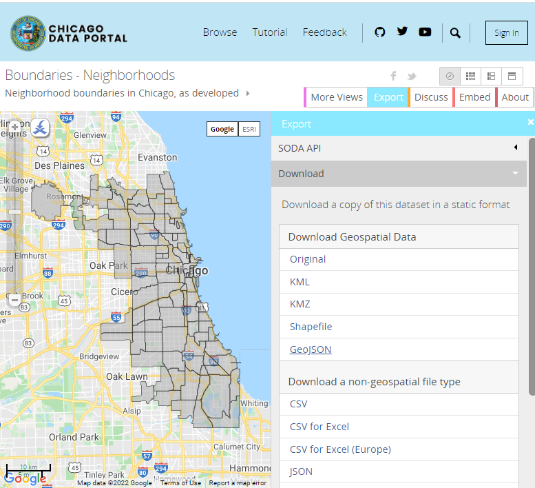
A copy of this dataset is also available in the project repository here.
1.2. Transform data
For this tutorial, we will use geojson.io to modify our GeoJSON file. If you navigate to this website and upload the downloaded 'Boundaries - Neighborhoods.geojson' file, this is how you will see the data in a tabular format.
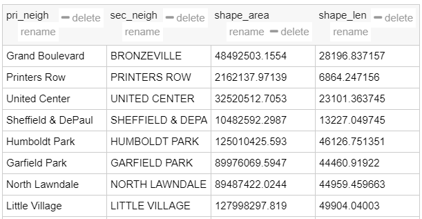
Notice how the tool automatically identified neighborhood boundaries. For now, we will only concern ourselves with the pri_neigh column which stands for 'primary neighborhood name'. This is the column that needs to match letter-for-letter to whatever neighborhood names that we choose to use in our main lead service line dataset factLSL.
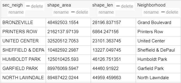
Let's go ahead and rename this column to Neighborhood for consistency. The modified GeoJSON looks like the image below. Go ahead and download this data as GeoJSON. You may overwrite the older file, if you wish to.
2. Service line material information (factLSL.csv)
2.1. Get data
To build a real map, service line material information must be available (lead or non-lead, both for public and private sides of the line). But in the absence of that, we can generate dummy data from the neighborhood boundary data that we have. Irrespective of whether we use real or dummy data, we need to generate a table named factLSL.csv and we want it to have the following columns and data types:
- Address (text): Property street addresses.
- Latitude (float): Latitude coordinate of the address location.
- Longitude (float): Longitude coordinate of the address location.
- LSLType (text): Descrption of the material used in the lead service line. You can choose to use any terminology that you prefer in this text column as long as the text indicates material used for both the public and private sides of service lines. We will see later how we can translate this information into something that our tool can understand.
- Neighborhood: Neighborhood of the address location.
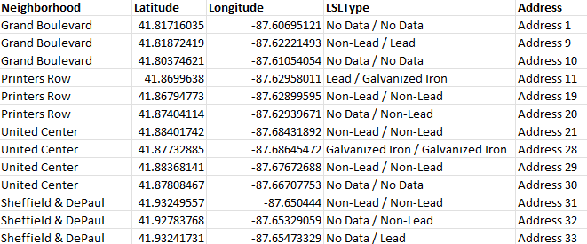
For the sake of this tutorial, we generated dummy data. The only restriction that we need to follow is ensuring that our latitudes and longitudes fall within the neighborhood boundaries. We used Python to do this, only so that we can generate hundres of dummy data points but you may choose to generate a spreadsheet manually. Feel free to use any tool that you want to for this purpose.
The data that we generated looks like this (image below).
3. Map line material to lead or non-lead (dimLSLType.csv)
You may choose to use any existing nomenclature to indicate the material that both parts (public or private) of the service line is made of. We choose the following nomenclature:
Examples:
No Data / No Data: No available data either about the public or the private side of the line.Non-Lead / Lead: Non-lead on the public side but lead on the private side.Lead / Galvanized Iron: Lead on the public side but galvanized iron (non-lead) on the private side.
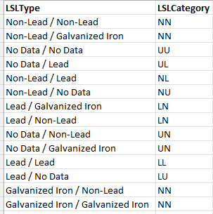
Using the table dimLSLType.csv, we map our custom nomenclature to a terminology that our tool can understand. Let's go ahead and make make sure that the mapping in dimLSLType.csv is as we expect.
For example,
- We want
No Data / No Datato map to "Public side unknown and private side unknown". The symbol for this isUU. - Similarly, we want
Lead / Galvanized Ironto mean "Public side is lead and private side is non-lead". The symbol for this isLN.
Here are the available symbols and what they mean -
NN: Non-lead on both sidesUU: Unknown material on both sidesUL: Unknown material on public side but lead on the private sideNL: Non-lead on public side but lead on the private sideNU: Non-lead on public side and unknown material on the private sideLN: Lead on the public side and non-lead on the private sideUN: Unknown material on public side but non-lead on the private sideLL: Lead material on both sidesLU: Lead on the public side but unknown material on the private side
If you are using the same terminology as we are, then your dimLSLType.csv will look like this -
Summary
So far, we prepared all the datasets that we needed for the final mapping tool to work! We should have these files under our Data path:
Boundaries - Neighborhoods.geojsonfactLSL.csvdimLSLType.csv
And one dataset that needn't change at all -
dimLSL.csv
That's all the data transformation there was. We have done all the heavy-lifting so far. In the next section, let's see how we can use these datasets to develop our maps.